Excel Geeking: Unwinding a Crosstabbed Dataset

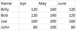
Sometimes you have to work with a data set that is not in a state conducive to, well, anything. I’m thinking specifically about crosstabbed data sets. More than once I’ve had to deal with a data set that looks like this:

Oh, if only there were a way to unwind this file so that it was in a more normalized state for querying, lookups, and general analysis.

Well, now there is.

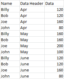
I created this routine a number of years ago because I had a monthly process that required taking a dataset like the one above and reformatting it into a layout that looks like this:

Needless to say, the data I was dealing with was a good deal larger than the sample above. I’ve used this routine on datasets that ended up outputting half a million rows. Yeah, it takes a few minutes, but it works. On smaller datasets, it works pretty fast.

Sub UnWindCrosstabData()
'   This takes a cross tabbed data and "unwinds" it to a flat file.

    ' Variable declarations.
    Dim rng         As Range
    Dim shNew       As Worksheet
    Dim lCols       As Long
    Dim lRows       As Long
    Dim i           As Long
    Dim j           As Long
    Dim r           As Long
    Dim vTemp       As Variant

    ' If the selection count is greater than one,
    ' assume a range to uwind has been selected.
    If Selection.Count > 1 Then
        Set rng = Selection
    Else
        ' Otherwise, use a range input box to get the range via the user.
        On Error Resume Next
        Set rng = Application.InputBox("Select the range to be unwound:", , , , , , , 8)
        ' If we get an error, the user did not select a range, and we exit the sub.
        If Err.Number <> 0 Then
            MsgBox "You need to select a range to use this utility.", vbExclamation, "Selection Error"
            Exit Sub
        End If
        On Error GoTo 0
    End If

    ' Get the total number of columns we will be dealing with.
    lCols = rng.Columns.Count

    ' Get the total number of rows we'll be dealing with, taking the use
    ' of headers into account.
    lRows = rng.Rows.Count - 1

    ' Speed up processing by shutting off screen flicker.
    Application.ScreenUpdating = False

    ' Set the new worksheet that will house the data.
    Set shNew = ActiveWorkbook.Worksheets.Add

    ' Reactivate the source sheet.
    rng.Parent.Activate

    ' Select and copy the source range, and paste it into the new sheet.
    rng.Select
    rng.Copy
    shNew.Activate
    ActiveSheet.Cells(1, 1).PasteSpecial xlPasteValues

    ' Reset the range to the pasted selection.
    Set rng = Selection

    ' Insert a column for the data header.
    rng.Cells(1, 2).Select
    Selection.EntireColumn.Insert

    ' Copy the record identifiers down, taking headers into account.
    For i = 1 To lCols - 2
        rng.Cells(2, 1).Select
        Range(Selection, Selection.Offset(lRows - 1, 0)).Select
        Selection.Copy
        rng.Cells(1, 1).Select
        Selection.End(xlDown).Select
        Selection.Offset(1, 0).Select
        Selection.PasteSpecial Paste:=xlPasteValues, Operation:=xlNone, SkipBlanks _
            :=False, Transpose:=False
        Application.CutCopyMode = False

    Next i

    ' Fill in the data header column.
    rng.Cells(1, 2).Value = "Data Header"
    r = 2
    For i = 1 To lCols - 1
        vTemp = rng.Cells(1, i + 2).Value
        For j = 1 To lRows
            rng.Cells(r, 2).Value = vTemp
            r = r + 1
        Next j
    Next i

    ' Insert a column for the data.
    rng.Cells(1, 3).EntireColumn.Select
    Selection.Insert Shift:=xlToRight

    ' Fill in the data.
    rng.Cells(1, 3).Value = "Data"
    r = 2
    For i = 0 To lCols - 2
        rng.Cells(r, i + 4).Select
        Range(Selection, Selection.Offset(lRows - 1, 0)).Select
        Selection.Copy
        rng.Cells(r + (i * lRows), 3).Select
        Selection.PasteSpecial Paste:=xlPasteValues
    Next i

    ' Delete the unneeded columns
    rng.Cells(1, 4).EntireColumn.Select
    Range(Selection, Selection.End(xlToRight)).Select
    Selection.Delete Shift:=xlToLeft

    ' Turn screen updating back on.
    Application.ScreenUpdating = True

End Sub

And having posted this, I’m already posting a hack. This routine only deals with one column of data to the left of your values. But what if you have more than one column? What if, for example, in the dataset above, you have name and address and city and state and zip code and email and phone number and…well, you get the idea.

What I do is to concatenate all of these fields together into a single column. I always use a delimiter, and for me, two good delimiters are the pipe (“|”) and the tilde (“~”). Once the field is concatenated and converted to values, I’ll run the routine above, then I’ll use Text To Columns to break all the columns back out again.

Use the above freely* and enjoy. If you have suggestion or find bugs, post in the comments section.

*and at your own risk, I assume no responsibility, legalese legalese legalese